Project Description
Abstract:
This project aimed to develop an automated tool to enhance traffic signal timing plans by detecting and correcting scheduling errors, a process previously conducted manually. After evaluating various machine learning algorithms, a 2D convolutional neural network (CNN) was chosen for its effectiveness in handling structured, grid-like data. Trained on a labeled dataset of signal timing schedules, the CNN model learned to predict optimal timing corrections, resulting in more realistic, consistent, and efficient signal schedules. With a focus on high accuracy and minimal computational overhead, the model achieved a 95% test accuracy and reduced correction time from five minutes per signal (manually) to an instant.
Introduction:
Traffic signal timing plays a crucial role in managing city traffic, as well-designed timing plans can improve traffic flow, reduce congestion, and increase road safety. In traffic management, timing plans define the specific signal settings, including the duration of green lights for each direction. The signal schedules are daily plans that specify which timing plan should be used at different hours of the day to match expected traffic patterns.
Miovision relies on these plans and schedules for its predictive traffic signal technology, often obtaining them from local transportation agencies. When these schedules aren’t available, Miovision generates predicted plans and schedules using vehicle GPS data. While effective, the generated schedules sometimes include small but noticeable errors, such as a single hour of one plan mistakenly inserted among consecutive hours of another - as shown in Figure 1. Manually correcting these errors takes around five minutes per signal—time-consuming work when thousands of signals require adjustment. The goal of this project was to use machine learning to automatically correct these errors, reducing manual work and speeding up the production of accurate timing schedules.

Figure 1. Example of a bad schedule
Methods:
The initial strategy for developing this tool involved fine-tuning a large language model (LLM) to understand the relationships between input schedules and corrected schedules. Given that the data was in JSON format, the idea was to input a bad JSON and have the model output a corrected JSON with adjusted values. Below in Figure 2, we present an example of one day from the input and output JSON. Note how the output schedule is simplified and more consistent across the days of the week.
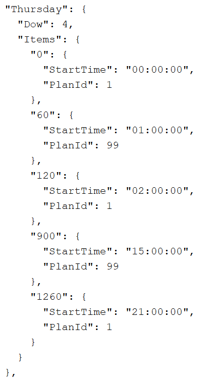
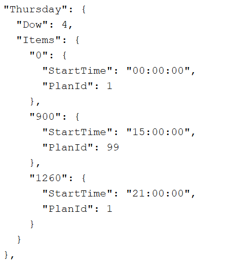
Figure 2. Comparison Between Bad and Good JSON
However, after fine-tuning the Llama 2 model using QLoRA, I realized that this approach would not be sufficient due to a lack of data. The dataset I had available consisted of only 350 example JSONs with hand labeled corrections as the ground truths. With this limited amount, the model struggled to generalize effectively to unseen test data. Additionally, the structure of the JSONs varied based on the specific schedules, which further complicated the model's ability to learn from the limited examples.
To gain deeper insights into the manual correction process, I consulted with operations employees to understand their approach. Although they followed certain guidelines, the presence of numerous edge cases made it impractical to create a simple rule-based algorithm. I learned that the ideal schedule could often be inferred by examining the hourly schedule and identifying the errors visually, such as in Figure 1. This methodology inspired me to approach the problem as a computer vision task, leading to the decision to use Convolutional Neural Networks (CNNs).
To do this, the first step involved building hourly schedules by constructing a 7x24 table for each traffic signal, representing the hourly schedule for every day of the week. This is to change the input from a JSON into a table like structure that mimics the visual that the employees look at when correcting manually. An example is shown below in Figure 3. The table was stored as a Pandas Dataframe
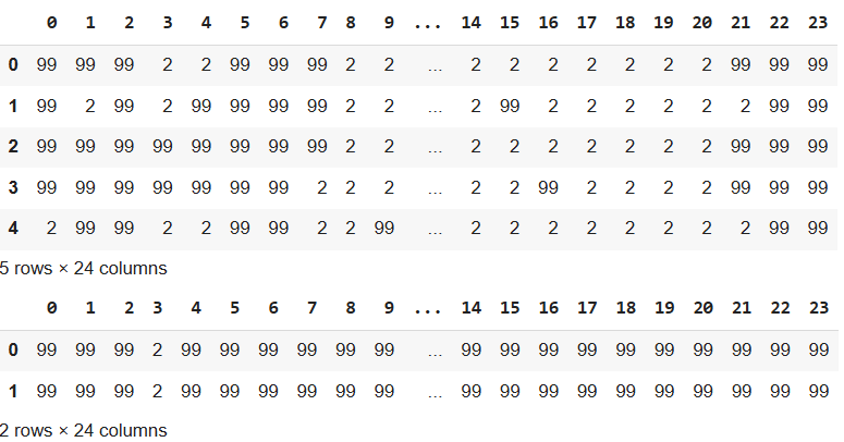
Figure 3. Example Schedule Dataframe
Then I created two CNN models using PyTorch, one for the weekdays that took in a 5x24 tensor as the input (5 weekdays & 24 hours) and one for the weekends that took in a 2x24 tensor as an input (2 weekend days & 24 hours). This is because one of the governing rules is that the weekday schedules must all be the same so instead of having the model treat each day as an independent schedule, it can capture interdependencies of all the weekdays and make predictions about a day based on the others. I applied a post processing step that had the plan for an hour of a weekday be the mode of that hour for all weekdays.
The CNN model architecture used convolutional layers to identify patterns in timing plan schedules and ensure consistency across weekdays and weekends. The model begins with three 2D convolutional layers, each extracting increasingly complex features from the 5x24 or 2x24 input matrices. Batch normalization is applied after each convolutional layer to stabilize training, while max pooling progressively reduces the spatial dimensions, focusing on the most significant patterns within each time interval. Following this, a fully connected layer compresses these features into a dense representation, and a dropout layer helps prevent overfitting. A final fully connected layer produces a flattened 5x24 or 2x24 prediction, which is then reshaped to match the desired output format for daily schedules. The output is then converted back into the appropriate JSON format. This architecture, tailored for detecting spatial dependencies within timing data, ultimately generates corrected schedules in a structured and interpretable format. A visualization of the general structure is shown below in Figure 4.
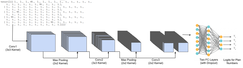
Figure 4. Architecture of Complete Model
One major challenge that still remained in developing this model was the limited dataset of only 350 examples. To address this, I treated the schedules like images and applied various transformations to generate a more robust and extensive dataset. By applying shifts, reflections, rotations, and adding random errors and noise to the schedule matrices, I expanded the dataset significantly, transforming the original 350 data points into over 200,000 synthetic examples. This enhanced the model's ability to generalize and improved its performance on unseen data.
Results and Analysis:
To train, I used a 90-10 training-validation split, and then tested the CNN models on a held out test set of 35 signals. I used accuracy at an hourly level as my performance metric, meaning a signal's accuracy was measured by how many plan's it got out correct out of the 168 hours of the week. The models achieved a test accuracy of 95%, effectively learning to distinguish between correct and incorrect timing plans. Compared to manual correction processes that took up to 5 minutes per signal, the model reduced correction time to instantaneous. Analysis of the results also showed a pattern amongst outputs that suggested signs of incorrect predictions. I added a post processing step to separate these predictions from the ones with high confidence to be later examined by a human.
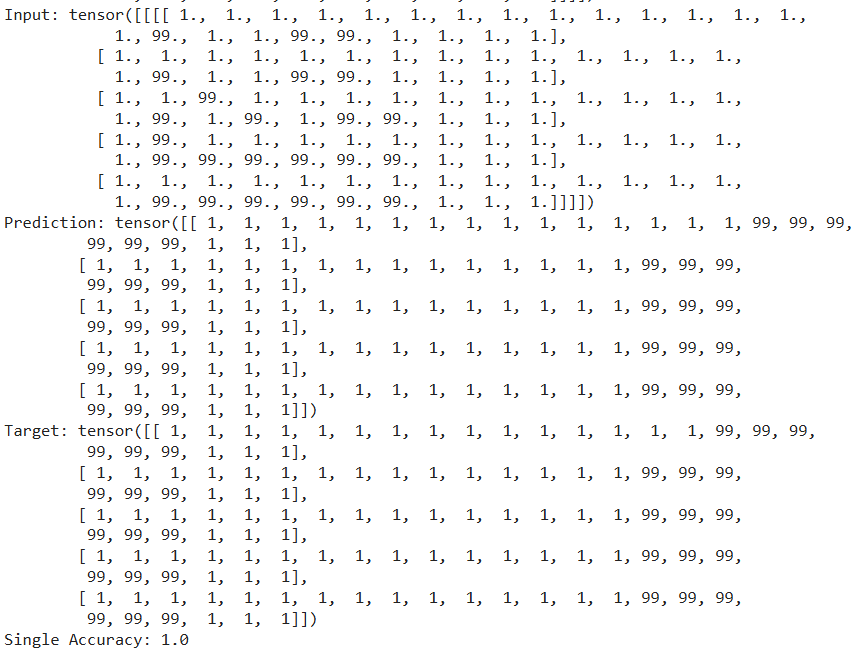
Figure 5. Example Output (Prior to JSON Conversion)
Personal Takeaways
Working on this project provided a practical application of CNNs in a domain outside traditional image processing. I learned how to adapt CNNs for structured non-image data, specifically for traffic management tasks, which broadened my understanding of model flexibility. Additionally, this project underscored the importance of data augmentation in generating a robust training dataset, as the initial sample size was limited, and increasing the number of training samples via data augmentation significantly improved model performance. Lastly, the most valuable takeaway is that I learned the importance of understanding the entire problem and starting out simple. Although LLMs initially seemed like the best solution because on how advanced and powerful they have gotten, understanding the problem and the manual process made me realize it was overkill and that simpler machine learning techniques were sufficient yet still effective. This not only led to better results, but saved computation time and power as GPUs were not needed for inference.